Posted by Sergiu Ciumac on August 01, 2021· 16 mins read
Posted by Sergiu Ciumac on August 01, 2021· 16 mins read
Why do you need video fingerprinting?
One of the most common use cases for audio fingerprinting is TV broadcast monitoring.
Generating detailed reports about aired TV content is done by analyzing its audio stream.
If you want to receive accurate statistics about the occurrence of a specific ad, applying audio fingerprinting may seem sufficient.
And indeed, it works in most cases.
At times though, advertisers use the same audio stream paired with modified visual content.
In the automotive and healthcare industries, it is actually widespread.
The visual content changes can be minor and sometimes even unnoticeable for the regular viewer.
However, it can play a big difference if you want to extract more information about the advertiser, the company, or your competitor.
Let’s start with a couple of examples to outline the problem.
Below is an example of a Toyota ad that uses the same audio stream paired with a different video.
Video 1. Four different commercial offers in a Toyota ad
The difference starts at the 10th second when the commercial offer appears on screen.
It stays on screen for 10 seconds, getting narrated to the audience.
Since advertisements are usually read fast and with the same tone of voice, audio fingerprints algorithms may fail to distinguish them.
The differences in the first examples are easy to observe.
Visual variations can be more inconspicuous though.
Take a look at some more examples in an increasing order of difficulty to detect the dissimilarities.
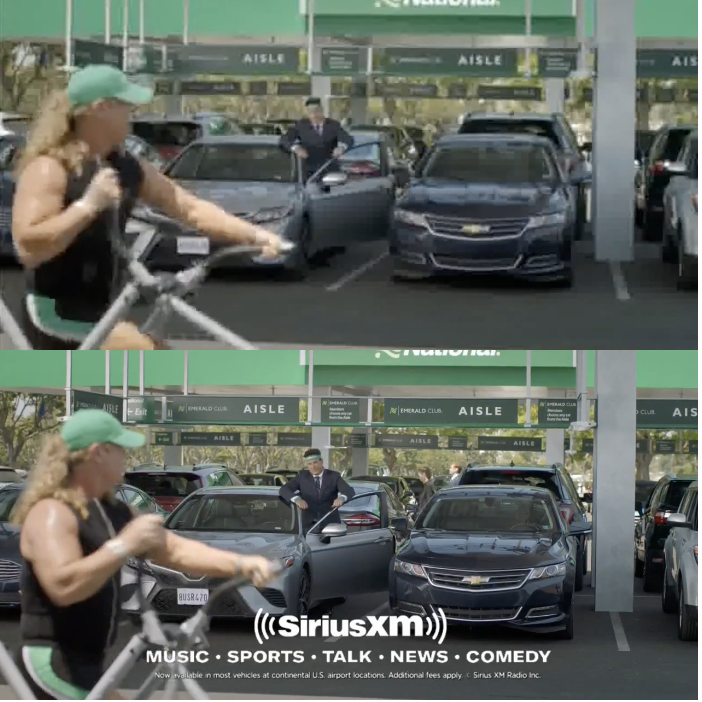
Video 2. National
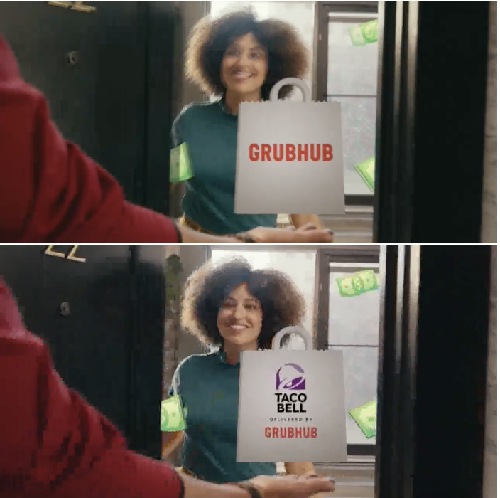
Video 3. GrubHub
For the “National” commercial, it is not difficult to spot the difference - SiriusXM text is present in the bottom spot but not in the top.
“GrubHub” is slightly more complex - the delivery bag contains two non-identical logos.
There is also one more distinction. Feel free to dig deeper into the ad to identify it.
The following two examples that are marginally different.
Try to identify the mismatches on your own.
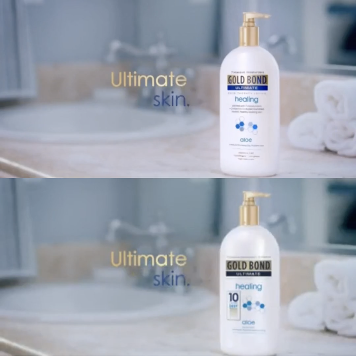
Video 4. Skin Lotion
Video 5. Prevagen
The skin lotion commercial contains two distinct bottles, more precisely different labels.
In the “Prevagen” ad, the logos on the exit screen mismatch - Walmart and GNC in the bottom right corner.
Also, for the automotive industry having different exit screens is quite common.
As they are aired in various regions, they contain specific dealership information.
Below is an example of the same commercial with six different endings.
Figure 1. Different exit screens of the same Toyota ad.
If you want to differentiate these ads, monitoring only audio content is not enough.
This is where video fingerprinting can help you.
Video fingerprinting
Similar to audio fingerprinting, video fingerprinting can be summarized in the following generic steps:
reducing the dimensions of the initial data points
extracting most relevant features from the downsampled data
encoding features into a format that is easy to retrieve and compare
The outlined problem had a couple more business-related constraints that we had to consider when developing the algorithm.
searching and comparing the ads have to be executed in real-time
real-time data feed comes from over 1000 TV stations, generating more than 24,000 hours of daily search content
search space is large - between 5,000 and 10,000 commercials.
So how do we approach this problem?
Firstly, video fingerprinting can be thought of as image search where the images are actual video frames extracted from the stream.
Every second of the video contains 30 color frames, which we can use as the reference points we want to retrieve and compare.
Those of you who read the description of the SoundFingerprinting algorithm may notice a pattern.
Audio fingerprinting uses image search techniques to search and retrieve similar spectrograms images.
Can we adapt the SoundFingerprinting algorithm developed for audio search to retrieve video frames?
It turns out we can.
Image search designed for spectrogram retrieval works remarkably well for video frames.
Dimensionality reduction
The first step in our algorithm is to reduce the dimensionality for the input video content: inserted ads and real-time queries.
The content is encoded in various formats, most commonly in 1080p HD widescreen format.
This resolution is far too big for the multidimensional search.
1920×1080 color vector is incredibly difficult to search.
If encoded in a one-dimensional array, its length is \(1920*1080*3 = 6,220,800\).
Conversely, modern approximate nearest neighbors search algorithms are benchmarked on vectors that have up to 1,000 dimensions.
Thankfully, we don't need this resolution to correctly identify the differences in the ads, so let's resize it to 128x72 pixel images. We found this resolution to be optimal after experimenting with a wide range of options. To give you an idea of how small it is, take a look at the video encoded in 128x72 format.
Video 6. National scaled to 128x72
At this resolution you can still distinguish essential details in the video.
The relevant information is preserved.
The corresponding step in the audio fingerprinting algorithm is downsampling. A high-resolution audio signal sampled at 44,1KHz is downsampled to 5,5KHz, retaining the most crucial bits of the initial audio.
A simple heuristic you can use to choose resizing parameters is to assert whether the information you are trying to differentiate is not lost in the process.
Asserting is relatively straightforward: visualize the downsampled files and make sure you can still see (or listen in the case of audio algorithms) the very thing you are trying to retain.
If you can’t see it anymore, chances are the information is irretrievably lost.
The next step in reducing dimensionality is encoding the color schema into a [0, 255] range. Keeping the original RGB is not required as a monochrome image preserves the original very well.
Video 7. National monochrome
The corresponding step in the audio fingerprinting algorithm is converting the original audio to mono sound.
After all these transformations, we have achieved a 675x dimensionality reduction.
Our vector’s length is now 9120.
Extracting features from images
Feature extraction from images is an incredibly reach domain of research.
Thankfully the problem we are trying to solve has a couple of advantages that make it easier.
Frames from a video have a stablescale and orientation.
We only operate with 128x72 images, which are never rotated on either of the axes.
This property greatly simplifies the task since feature extraction can be done much faster for this type of image.
What are the features that encode important information about the image?
One of the essential abilities of the human eye is detecting and differentiating shapes.
Stripped to its core, every shape is made of edges.
As an example, think about an image of a clear blue sky.
It has almost no information: all pixels are of the same value.
Now imagine a white plane in the blue sky.
This new image contains edges created by neighboring pixels of different values, white and blue.
The presence of these edges adds information value to the picture.
It suddenly becomes more meaningful for the observer.
That is why edge detection is such an important area of study in computer vision.
Take a look at what happens when one of the video frames is convolved using a simple filter designed for edge detection.
Figure 2. Simple edge detection convolution applied on one video frame.
It removes all the non-essential bits from the image, leaving us with shapes that our brain interprets as meaningful - the Toyota logo and English letters.
Arguably, the most essential features of an image are edges.
Finding an algorithm that focuses on efficiently encoding edges in a feature vector is the main challenge of our task.
2D Discrete Haar wavelet transform
The Haar transform is the simplest orthogonal wavelet transform.
It operates over \(J=log2(n)−1\) scales, computing a series of coarse-scale and fine-scale coefficients on the input image.
What does it mean to compute multiresolution coefficients, and why do we need this?
A more straightforward explanation, discrete Haar Wavelet transform is one of the simplest methods to find edges in an image.
It identifies them on \(J\) smaller scales.
For instance, an image that is 512x512 pixels in size will generate coefficients for 8 coarse scales.
Decreasing the resolution of an image is a neat trick to retain the most prominent edges.
You can get an idea of what image resolution decrease means by looking at the following example of a video frame after discrete Haar Wavelet transform was applied to it1.
Figure 3. Standard Haar Wavelet decomposition applied on one video frame.
A curious reader might notice that the applied transformation is a standard wavelet transform where all the rows are processed before all the columns.
This decision was deliberate as it proved to work well for others.
The result is quite telling.
You can notice how on each step edges are detected on a smaller and smaller resolution.
In the quest of reducing the number of dimensions of the original vector, wavelet coefficients gave us a powerful mechanism.
The last step we use in image processing is filtering wavelet coefficients by their magnitude, keeping only a handful of them.
By retaining top wavelet coefficients, we can encode the most important features from the image.
After extensive experimentation keeping 4% of the original vector of wavelet coefficients provided the best precision/recall ratio.
Locality Sensitive Hashing
After reducing the original image frames to a vector of 9120 floats, out of which only 365 values are not zeros, we can apply approximate nearest neighbors search techniques to finally encode our frames in a format that is easy to search and retrieve.
Similar to audio fingerprinting, we treat our sparse vector of top Haar wavelet coefficients as a set.
How can we treat a vector of real numbers as a set?
Quite simple - we encode the sign of the top-wavelets to 10 (positive) and 01 (negative)2.
By applying this trick, we transform our wavelet coefficients array to a boolean array of length 18,240.
As a result, this decision enabled us to use the Jaccard Index as the distance metric when comparing two sets for similarity3.
Jaccard Index as a metric of similarity between two sets. The more similar they are the closer it is to 1.
LSH applied on sets is quite different from random projections that are used in Euclidian space.
I encourage you to read how LSH was used for audio fingerprinting, as I provide a more detailed explanation of why random min-hash permutations are equivalent to random projections when the Jaccard distance metric is used4.
How many min-hash permutations are needed to achieve a working LSH schema?
Similar to audio fingerprinting we use 100 min-hash permutations to generate random set permutations.
It worked great for spectrograms, so we decided to use the same number of permutations for video frames.
These 100 min-hash permutations will group resulting hashes into 25 hash tables with 4 permutations per table.
Chosen parameters may seem arbitrary, but they are not.
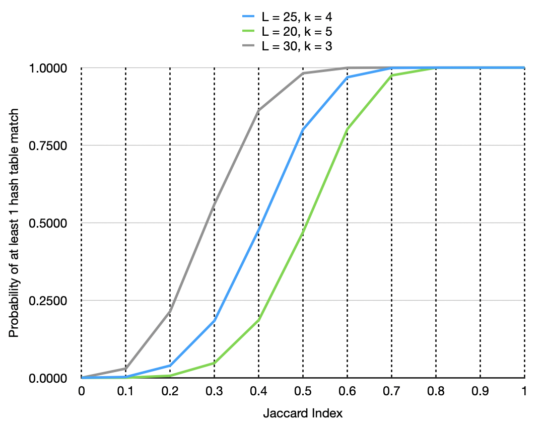
The probability that min-hash permutations will agree at least in one of the hash tables is given by the following formula5:
\[P = 1 - (1 - J^k)^L\]
where \(J\) is the Jaccard Index, \(k\) is the number of min-hash permutations in one hash table, and \(L\) number of hash tables.
Figure 4. Probability of at least one hash table match increases with similarity of the data points.
Notice how the probability of at least one successful match works almost like a step function.
When the similarity of two sets crosses the 50% mark, the probability of at least one successful match increases dramatically.
This is precisely what we need.
Filter out the noise and get good candidates only when they are similar.
We have chosen \(L=25\) and \(n=4\), as this schema is more forgiving, returning more candidates from a search request.
This trade-off was driven by the specifics of the video frame matching.
As video streams come from various sources, they are encoded in different formats: 4:3, 16:9, 1:1
When transforming it to a canonical format, transformation artifacts are inevitably introduced: pixelation, aliasing.
You don’t want to have an algorithm susceptible to these issues.
Thus a more lenient LSH schema is preferable.
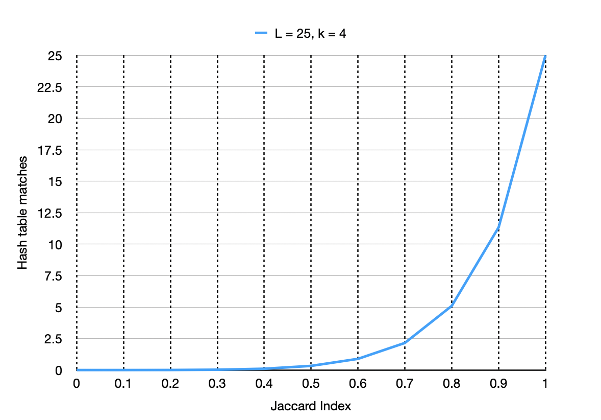
To control how sensitive the algorithm is, you can also consider only those candidates that matched in more than just one hash table.
Figure 5. Choosing how many hash table have to match for a point to be considered a candidate
Notice how with the increasing similarity, the number of matching hash tables increases as well.
In simple terms, if you need to analyze only those images that are 80% similar, you can retrieve only those candidates that match in at least 5 hash tables.
Matching Video frames
I’ve started this article with an example of different Toyota offerings getting injected into the same ad.
How do we spot these dissimilarities using the algorithm outlined above?
We start by sending real-time video stream queries to our Emy storage cluster.
Since each second contains 30 frames, 30 query points are used to retrieve potential candidates.
We get a set of matched frames and reconstruct the best matching path for every advertisement.
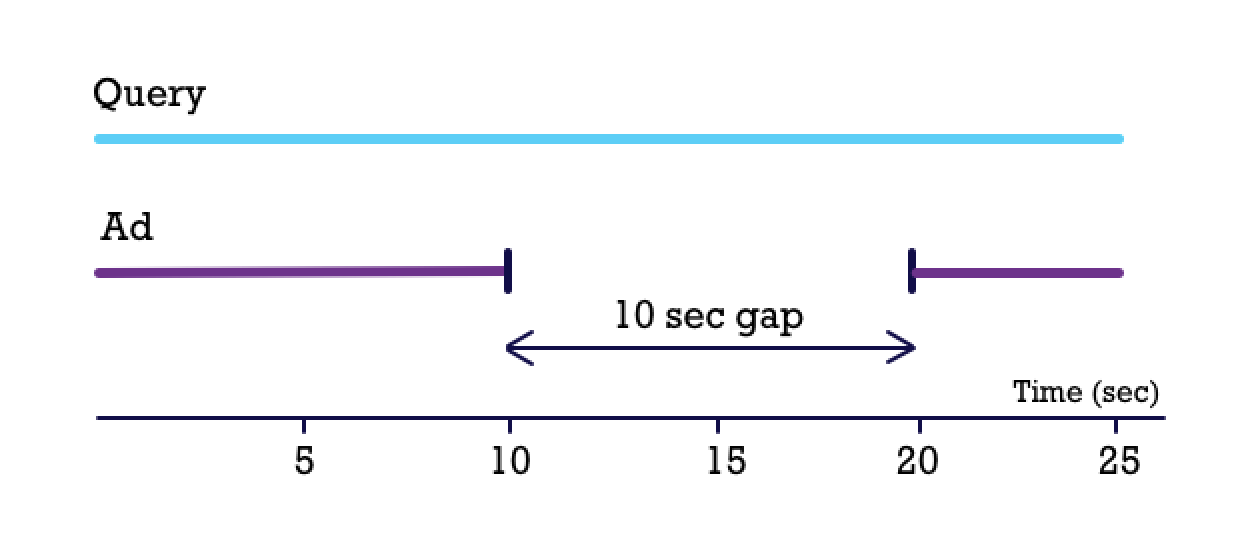
Once reconstructed, we use it to detect gaps in the resulting ad.
Areas where a gap is detected, identify the video frame differences.
For the first Toyota example, different commercial offers generate a 10 seconds gap with the original.
Figure 5. Created gap marks ads as different
I will leave the details about how the best path is reconstructed from the resulting frames for a different article.
It is on its own a complex problem to solve, essentially a variation of the edit distance problem6.
Detecting smaller details
What about use cases when the original and query ads have insignificant distinctions - i.e., different logo or phone numbers.
Provided LSH algorithm will not differentiate between them, it will not generate gaps in the reconstructed best path.
This is expected: we can’t make LSH + Min-Hash act as a precise retrieval algorithm since it is, by definition, an approximate nearest neighbor search.
To be able to detect small changes, stage 2 verification had to be implemented.
After the best matching path is reconstructed, we apply a simple frame-to-frame comparison that compares the differences on the pixel level.
For the frame-to-frame comparison, our first choice was the SSIM method.
SSIM is a metric that is used to measure image quality, but nothing stops us from comparing frames that match via LSH.
Since it is designed to detect noise and compression artifacts, it also can detect minor differences in the image very efficiently.
The problem with SSIM is that computation-wise, it is very expensive.
Applying it to a real-world solution that filters thousands of ads on hundreds of TV stations is not feasible.
In search of a faster approach, we decided to use a simple difference of gaussians between images to identify areas that contain different visual content7.
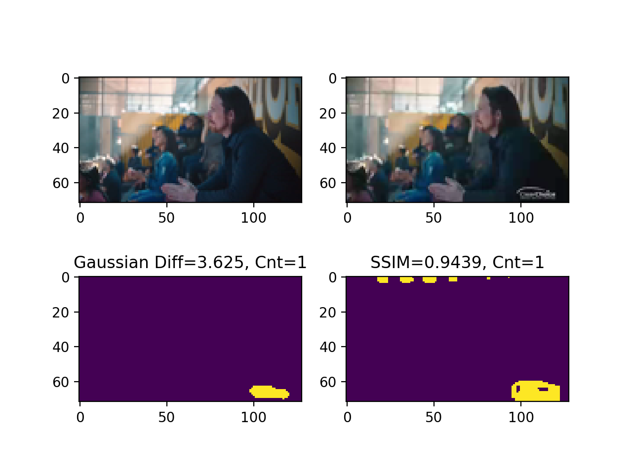
Take a look at the following examples with a side-by-side comparison of SSIM and the difference of gaussians.
Contours are colored in yellow to outline exact regions where the source and the target images are distinct.
Figure 6. Gaussian vs SSIM both detecting a missing logo.
Notice how both of the algorithms correctly identified a missing logo on the bottom right.
SSIM also identified additional changes on top of the image.
These are compression artifacts present in one of the videos.
They appear when different video formats are used to encode the video stream.
The difference of gaussians ignored compression artifacts, making it a better fit for the task.
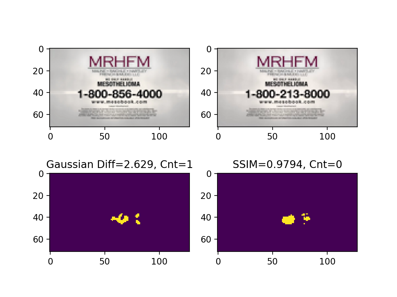
The following example contains video frames with two different phone numbers, everything else being equal.
Both algorithms identified the mismatch with ease.
Figure 7. Gaussian vs SSIM both detecting phone number differences.
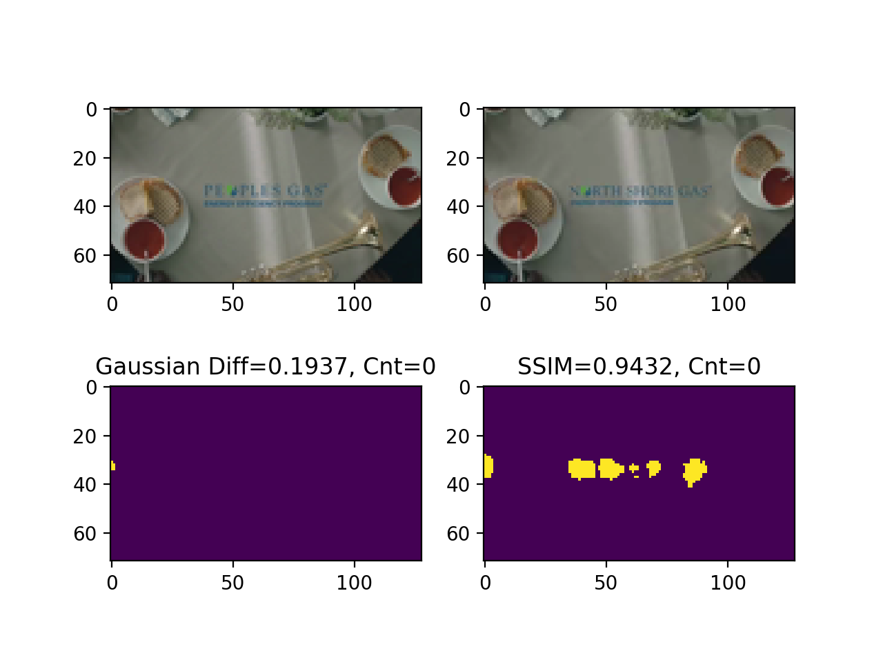
As a final example, I will show when the SSIM method fares better.
Notice how the difference of gaussians could not spot distinct company names: “Peoples Gas” vs. “North Shore Gas.”
Figure 8. Difference of gaussian not able to identify different company names.
It is not difficult to explain why this happened.
After applying a Gaussian filter on the frames, letter pixels blend with the background, as the color of these pixels is similar.
This is a limitation of the difference of gaussians - if the distinction blends with the background, then the algorithm will fail to identify it.
Nevertheless, I decide to stick with it provides an excellent trade-off between performance and precision.
The final step in stage 2 verification eliminates frames from the best-reconstructed path containing contours identified by the algorithm
Once these frames are eliminated, the best path will have gaps.
Gaps provide the time location where the video starts to mismatch.
Results
Watch the following examples of best-reconstructed paths with frame-by-frame comparisons identifying mismatching contours.
A stable contour will be detected in the first one on the 15th second when SiriusXM text appears.
Figure 9 shows one of the frames when the difference starts to appear.
Video 8.National ad differences.
Figure 9. SiriusXM difference.
Notice how at times, contours are identified not only during SiriusXM appearance.
A fast motion may be the cause of an imperfect best path alignment between query and track frames.
Nonetheless, this is not a cause of concern.
It is enough to have at least 1 frame out of 30 during 1-second playback to get correctly aligned to prevent accidental gap creation.
The next example shows how the contour is detected on the lotion bottle at the ad’s middle and end.
Video 9. Skin lotion with different bottle labels.
Figure 10. Missing 10 on the label.
The last one is GrubHub with different logos on the bag.
Video 10. GrubHub with different logos.
Figure 11. Taco Bell logo on the bag.
Using it in production.
After developing and integrating a video fingerprinting algorithm, Emysound can now fingerprint, search, retrieve, and compare both audio and video streams in the same processing pipeline.
Video fingerprinting is now used to identify between 3,000 and 6,000 ads displayed over 1,000 TV stations.
Using LSH + MinHash allows us to search through over 25,000 hours of both audio and video content.
Video fingerprinting algorithm is implemented in the same open-source solution as audio fingerprinting: SoundFingerprinting.
I haven’t had the time to update the GitHub page with hands-on examples of programmatically generating video fingerprints though I will do it in the upcoming months.
If you are interested in using it drop me a line.
To support my efforts in developing SoundFingerprinting further, please star the project on GitHub.
The core fingerprinting algorithm is MIT licensed, so you can use, change, and distribute it freely. Sign up for Emysound if you are interested in using content recognition services for a commercial project.
1 - The resulting image contains more than log2(n) scales because applied method is a standard Haar wavelet transform.You can learn more about the differences in the way a 2D Haar wavelet transform is applied here.
2 - Using the sign of the wavelet coefficient proved to work in the past - C. Jacobs, Finkelstein, A., Salesin, D. (1995) Fast Multiresolution Image Querying. Proc. SIGGRAPH.
3 - Jaccard similarity and min-hash values have a powerfull relationship where the probability of min-hash match is equal to Jaccard index. More details here.
4 - From CS246 Mining Massive Datasets, slides can be found here.
5 - If you want to get an intuitive view of LSH applied in Euclidian space, I would recommend this article as an introduction. The author hashes the points using random rotation as a random projection which is a neat trick used o build visually intuitive partitions.
6 - One of the most common algorithms that try to align temporal sequences is known as Dynamic Time Warping. Solutions for edit distance problems are more generic, and can also be applied in the corresponding context.
7 - The only change from the original difference of gaussians algorithm is that we use the same sigma for both images.