Posted by Sergiu Ciumac on June 12, 2020· 23 mins read
Posted by Sergiu Ciumac on June 12, 2020· 23 mins read
Audio Fingerprinting
I have been developing the SoundFingerprinting open source project for the last ten years.
One of the questions I often receive is “how does music recognition works?”
For the library users, it is somewhat similar to a one-way hash function.
You provide a file at the input, and after a certain number of conversions, you get “audio fingerprints” at the output.
Looking at the actual values of these fingerprints, they are entirely opaque.
The question begs: What information do these integers contain?
My goal in this article is to dissect the algorithm’s two main steps: compression and hashing.
Additionally, I will explain why audio and image search are so intertwined.
Compression and Hashing
Compression - from Latin comprimere press together
From a higher level, all audio fingerprinting algorithms go through two transformation steps: lossy compression and hashing.
We want to preserve as much relevant information as possible with the smallest footprint.
Look at the following array:
// ten entries of 1int[]data={1,1,1,1,1,1,1,1,1,1}
We need at least 40 bytes to store it 10*sizeof(int).
In practice, a data point $P$ has two fundamental properties that influence how fast you can find it in a database of similar points.
That is the size and data format.
\[SearchTime(P) \sim Size(P) + DataFormat(P)\]
Let’s try to compress the array.
The first step we can apply is a simple Huffman Encoding that allows representing the same amount of information more compactly:
// the value of one repeats ten times.intval=1,repeat=10;
Now it uses 8 bytes: 2*sizeof(int), a 5x reduction.
Good step forward on the size side, but what about the format?
The format is still clunky, so let’s encode it into one long:
// tuple with 2 integer values (1, 10) gets encoded into one longlonghash=(1L<<32)+10;// value of hash is 4,294,967,306
After these steps, we have one variable that holds exactly the same amount information in a much more convenient format. Why is it convenient?
it is compact, storing 1000 of similar sequences requires 5x less space
it is sortable, you can search an entry within \(log(N)\) steps, where N is the number of stored entries.
On a higher level, Audio Fingerprinting algorithms try to achieve a similar goal: Convert an audio signal to the most compact and convenient format for storing and searching.
Notice that the above conversion is an instance of lossless compression.
You can completely restore the initial sequence from the final value:
intrepeat=hash-(1L<<32);// 10, how many times to repeatintval=(hash-repeat)/(1L<<32);// 1, the value to repeatint[]data=Enumerable.Repeat(val,repeat).ToArray();// initial data
Audio Fingerprints do not require lossless encoding.
You don’t need to reconstruct the original signal knowing the fingerprints.
The only requirement is fingerprints with the same value should come from the same or similar sound.
Since we don’t need to reconstruct initial data, we can apply a different last transformation step on the tuple (1, 10).
it is even more compact = 2 bytes, 20x reduction from the original size.
it is convenient to store as a simple string.
Hashing has its own cost.
You can’t reconstruct original tuple since you don’t know if "11" is 1 that repeats ten times, or is it 9 that repeats 2 times.
Even more so, we have 10 other tuples that hash into the same value of “11”.
These are called hash collisions.
Audio Fingerprints are similar.
Some of them are equal because they come from the same source, others because of a random hash collision.
How to compress an audio signal
There is a wide variety of file formats mp3, ogg, flac, all of them generating different byte representations.
All fingerprinting algorithms decode the input file into a raw wav format first.
SoundFingerprinting is no exception.
Once we decode the audio file, we can focus on the following properties of the audio track:
number of channels - mono, stereo or other
sample rate - typically 44,1KHz
bit depth - 8, 16 or 32 bits per sample
If we have a one-minute audio file, sampled at 44,1 KHz with 32 bits per sample, we need 21,168,000 bytes to store it: 2*60*44100*32/8.
It amounts to 20MB of storage for just 1 minute of audio content.
The following compression steps minimize the size of the data 32x fold:
stereo to mono - 2x reduction
44KHz to 5,5Khz - 8x reduction
32 to 16-bit depth - 2x reduction
The same 1-minute file now has 661,500 bytes ~0.63MB.
It is an example of lossy compression.
We are essentially getting rid of the rich quality in favor of a more compact format.
Perceptually, we can still hear the sounds and differentiate them.
It is just not as sharp and clean for regular use.
Below are some examples of the compressed formats1:
Sound
Channels
Sample Rate
Bit Depth
Size Reduction
2
44.1KHz
16
1
44.1KHz
16
2x
1
11KHz
16
8x
1
11KHz
8
16x
1
5.5KHz
8
32x
Table 1. Let Me Call You Sweetheart in different audio formats
What acoustic information we want to preserve?
Even after all these compression steps, the audio signal does not show any improvement in format convenience for storing and searching goals.
// one minute mono file encoded in 8 bit depth sampled at 5512Hz// is just an array of bytes of 330,720 lengthbyte[]audio={1,2,3,4,5,6...}
It is still unclear how you can search for a 10-second snippet picked at any location from this audio signal.
// search querybyte[]query={1,2,3,4,5,6...}// length of the array 10 * 5512 = 55,120 elements.
Even if you correctly align the query snippet in the original file, element by element comparison will not work.
It is enough to increase the “loudness” in the query snippet by any factor, say 1.25x, and all your array values in the query will increase by the same factor - 1.25x.
As expected, Audio Fingerprinting algorithms should be resilient to sound intensity increase or decrease, as well as noise.
All audio fingerprinting algorithms handle this challenge by treating the sound as a spectrum of frequencies.
Sound is a pressure wave conveyed through some medium like air or water2.
Two tones are similar if the wave that describes them is similar.
The content of an audio signal array is just a discrete version of that wave.
If we are sampling at 5512Hz, we describe each second of the sound with 5512 samples.
To better understand how discretization works, see how it works for yourself.
Figure 2. Sample a 1Hz wave at 10Hz rate
The graph shows how 1 second of an audio signal is sampled in 10 points.
Technically, we sampled the signal at 10Hz rate.
The signal itself is just a pure tone since it is composed only of one function: \(sin(x)\).
Notice how the sinusoid completed 1 full cycle in 1 second on the y-axis.
It means that the sound wave vibrates with a frequency of 1Hz.
The file that you would like to fingerprint can be sampled at any rate, SoundFingerprinting will downsample it to 5512Hz.
We didn’t pick 5512Hz at random.
Within a discretization rate of 5512Hz, according to Nyquist–Shannon theorem, we will be able to capture frequencies from 0 to 2756Hz.
The theorem states that for a given sample rate \(f_{s}\) perfect reconstruction is guaranteed possible for a band limit \(B<f_{s}/2\).
A healthy auditory system can capture frequencies between 20 to 22KHz. Why do we disregard such a big range [2756Hz, 22000Hz]?
Mostly because we trade high frequencies for a smaller footprint, moreover, out of the available frequency range [0Hz, 2756Hz], SoundFingerprinting takes into account only the domain between [300Hz, 2000Hz] filtering the rest.
Arguably, this range proved to work best for the task3.
You can play with the pure tone generator to get an idea of which frequency components are filtered and which ones are left.
Figure 3. Pure tone generator
In case you are familiar with the exact nature of the fingerprinted sound, you can change this range to include more frequency components.
One more reason to fingerprint only a fixed frequency range relates to musicology. Musicians often use A4 as a central note when tuning their instruments.
The modern concert pitch for this note is 440Hz, which aligns well with the fingerprinted range.
Note
Frequency Hz
A4
440
B4
493
C5
523
D5
587
E5
659
F5
698
G5
783
A5
880
Table 2. Notes tuned around A4 at 440Hz frequency
From the auditory system perspective, different musical instruments can sound different even when playing the same note.
It happens because of the harmonics that they emit alongside the pure tone.
Harmonics are additional frequencies that lie at multiples of the fundamental frequency. An instrument that plays A4 generates 440Hz pure tone and harmonics at 880 Hz, 1320 Hz, 1760 Hz.
Click to play an example of A4 that plays as pure tone (0-5 seconds), then with odd harmonics (5-10 seconds), then will all harmonics (10-15 seconds).
Figure 4. 440Hz sound as pure tone 0 to 5th second, with odd 5th to 10th second and all harmonics 10 to 15 second
From the fingerprinting perspective, we are not very interested in high-end harmonics.
They are undoubtedly important for our perception but not critical for pattern recognition tasks.
That’s why we filter them.
Similarly, low-end bass frequencies are usually capturing environmental noise.
Check a typical airplane noise.
Figure 5. Airplane noise doesn't enter fingerprinted range
Since we start fingerprinting above 300Hz, whatever is lower is filtered, not affecting generated fingerprints.
Let’s take a look at a typical 15 seconds conversion between two people.
White lines outline the frequency band, which is used by default by SoundFingerprinting library to build audio fingerprints.
Figure 6. Spectrogram of a conversation. White horizontal lines outline the range used for fingerprinting [300Hz, 2000Hz].
The brighter is the area, the more acoustic information is present in the frequency ranges shown in the image.
In other words, we are mostly interested in frequency peaks that contain the most relevant information we would like to preserve (shown in white).
Figure 7. White areas contain most valuable acoustic information we want to preserve.
All audio fingerprinting algorithms are hunting these peaks, with various techniques and approaches.
Overview of image search
Once we’ve identified what kind of information we would like to preserve, the main challenge is encoding it in an efficient format for storing and searching.
If we look at the previous spectrogram examples, they can be treated as three-dimensional objects:
x-axis - time in seconds
y-axis - frequency in Hertz
the amplitude of the frequency - the intensity of the color
The most intuitive way to encode this information is simply in an image.
At this stage, many people are getting confused.
We are transitioning from an audio domain to a visual domain simply because there is no better way to encode a spectrogram than in an image.
Similar spectrogram images bear similar sounds.
Notice how image search algorithms try to solve a similar problem:
identify features which best describe the image
encode identified features in an easy to use format for storing and searching
Most sophisticated image search algorithms are constrained by the requirement of being scale and rotation invariant.
Let's take ORB1 as one of the feature extraction algorithms.
ORB builds a set of keypoints from the image, which are preserved even if the image is scaled or rotated.
1. ORB - Oriented FAST and Rotated BRIEF, alternative to SIFT and SURF in computation cost, matching performance and mainly the patents.
Figure 8. ORB keypoints preserved during rotation and scale
This property is incredibly useful for various use-cases but, at no surprise, comes with computational costs.
Fortunately, we do not need features that are immune to scaling or rotation.
Spectrogram images have an advantageous attribute: their scale and orientation is stable.
Extracting features from such images is much easier.
The height of a spectrogram image equals to the frequency resolution.
Y-axis is encoded in 32 log-spaced bins, which yield 32 pixels.
The width is chosen empirically.
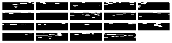
Figure 9. 19 spectrograms cut from an audio file each 128x32 pixels in size
Since x-axis in a spectrogram corresponds to the time domain, the width of an image is equal to the length of the cut in seconds.
SoundFingerprinting uses 8192 audio samples per fingerprint, which corresponds to 1.48s.
The spectrogram uses 64 samples overlap, meaning the intensity of one pixel corresponds to the frequency resolution of 11.6ms.
It yields an image that is 128x32 pixels, where every pixel is between 0-255 range.
These parameters may be quite confusing if you are reading them for the first time.
Don’t worry, just keep in mind that the spectrogram image is essentially an interpretation of how sound frequencies change over time.
We could have easily chosen a shorter timespan, say 4096 samples.
In this case, the width of the image would have been 64 pixels.
Choosing these values is a matter of parameter tuning.
To summarize, the images we are trying to detect are of the same size and orientation.
Features that make them unique are spectrogram peaks. So how do we encode them?
Encoding Image Features
Even though we have compressed relevant acoustic information of 1.48 seconds into the 128x32 image, it is still not an easy format to search.
A vector of size 4096 is just too big for the task.
// every image is 4096 bytesbyte[][]images=GetSpectrogramImages(audioFile);
To give a perspective, one descriptor in the ORB algorithm is a byte vector of length 32.
It makes them quite easy to search in a vast database of descriptors.
Since the focus is on frequency peaks, one easy way to reduce the dimensions of our image but keep the peaks is thresholding.
The thresholding methods replace each pixel in an image with either:
a black pixel if the image intensity \(I_{i,j}\) is less than some fixed constant T
or a white pixel if the image intensity is greater than T.
Thresholding gives the advantage of getting a very sparse representation of the same byte array, with intensity either 0 or 255, which can be easily encoded as booleans 0 or 1.
Figure 10. Thresholded spectrogram images. Threshold T equals to 165, resulting intensity values encoded as 0 or 1
Query images that are having white contours in the same image coordinates can be treated as similar images, thus similar sound.
One other approach is instead of thresholding the image, we can use Haar Wavelets to achieve a similar goal: identify frequency peaks.
Haar Wavelets have been successfully used in image search for quite some time4.
One naive approach when searching a spectrogram image in a database of stored fingerprints is to iterate over all them comparing one by one.
It will take \(N^2\) comparisons, and soon will become unfeasible even for a database that contains few images.
To give a perspective, 1000 hours of audio content will generate around 38 million fingerprint images.
Thankfully, there has been significant progress in the Approximate Nearest Neighbor Search in the last years5.
Let us analyze locality-sensitive hashing.
Hashing with Locality Sensitive Hashing
The origin of the word “locality” is “localis” - from French localité or late Latin localitas, from localis ‘relating to a place’
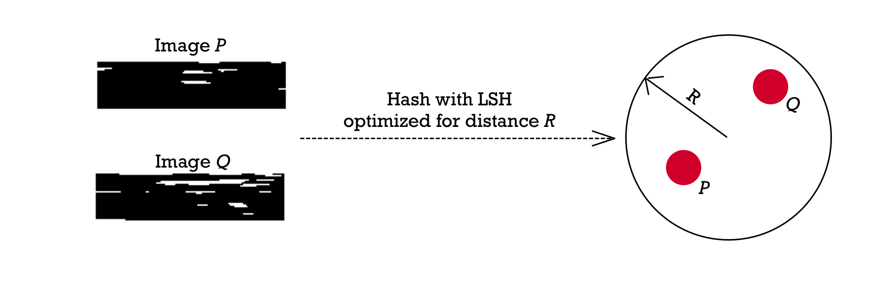
Locality Sensitive Hashing is an algorithmic technique that tries to build a forgiving hash data structure.
Its primary purpose is to ignore small differences between close points and hash them into the same bucket.
All the points that are “related to the same place” should have an equal hash.
Figure 11. Two images hashed in two points within distance R
One of the most important choices we need to make when designing the LSH data structure is defining the distance metric.
In other words, how sensitive our hash function should be to the proximity of the data points?
In the SoundFingerprinting case we can take advantage of the two things:
the 0,1 domain, our feature vector is a bit-vector
the sparsity of the data
Knowing these properties allows us to treat our images as sets.
And for sets, we can use the Jaccard Coefficient as our distance metric.
I've always found it difficult to explain how sets can be partitioned using locality sensitive hashing.
Let me explain what kind of LSH techniques are used for geometric spaces first.
Geometric vectors are much easier to visualize since we can use the Euclidian distance2 function to denote proximity between points.
2. Euclidean distance or Euclidean metric is the "ordinary" straight-line distance between two points.
Ideally, we want to partition our points into different hash buckets such that only those points related to each other, hash into the same bin.
Figure 12.p' and q' hash into the same bucket
Unfortunately, this type of perfect partition is not attainable.
Designing an ideal partition function will take longer than doing a simple element-by-element search through the entire dataset3.
3. Similarly how k-means clustering is a NP-hard problem.
To solve this problem, researchers have introduced randomized partitioning.
For each different randomized partition, the points will hash into different hash buckets, creating different hash indexes.
Figure 13. Three different partitions create different indexes
The number of randomized partitions governs the probability of getting a successful match \(p\) from a similar query point \(q\).
Since we can’t have a perfect partitioning, LSH data structure will give us a probability of a successful match, with respect to how many partitions we take.
The size of the dataset and the points’ dimensions govern the number of random projections.
Generally speaking, the more partitions you take, the higher the probability of a successful match between points that are within close distance.
A curious reader might ask why we haven't chosen Hamming distance4 as we are already operating with binary vectors?
The reason is that the resulting images are very sparse6.
Consider two completely zeroed spectrogram images (p,q) (that is, full or partial silence).
The Hamming distance between the two will be zero, reflecting complete similarity.
4.Hamming distance between two bit-vectors measures number of positions with different bit values
We should not treat silence as a similarity signal.
It can produce too many false positives, as any recorded discussion is full of small pauses.
That’s why choosing the Jaccard Coefficient is a better choice.
Comparing to a Hamming distance, two spectrograms with complete silence will have a Jaccard Coefficient equal to 1, signaling total dissimilarity.
Jaccard Coefficient as a distance metric
Jaccard Index is a statistic used for indicating how common two sets are.
It is defined as Intersection over Union of measured sets.
\[J(Q,P) = \frac{|Q \cap P|}{|Q \cup P|}\]
As an analogy, think about how a book store can treat a profile of their customer.
A profile may contain a set of past purchased books out of all available titles: bool[] purchasedBooks.
Every index of that bit-vector would map to a particular title.
For example, purchasedBooks[2] would tell us if the customer bought the third title in the bookstore.
To compare two different customer profiles, we could easily count how many values of 1 are in common between these profiles and divide it by the total number of purchased books.
publicdoubleCalculateJaccardIndex(stringcustomerProfileP,stringcustomerProfileQ){bool[]q=GetProfile(customerProfileP);// get customer profilebool[]p=GetProfile(customerProfileQ);// get customer profilevarzipped=q.Zip(p);intintersection=zipped.Count(tuple=>tuple.First&&tuple.Second);intunion=zipped.Count(tuple=>tuple.First||tuple.Second);if(union==0)return0d;return(double)intersection/union;}
The more values of 1 are equal, the more likely these customers have the same book preferences.
Not surprisingly, this is how many recommendation engines work.
Google used this metric to personalize visitor’s news feed.
To turn the Jaccard Index into a distance metric we can use its complimentary.
It is known as the Jaccard Coefficient.
So for two customer profiles with the same list of purchases, the Jaccard Coefficient will be 0, meaning they bought the exact same titles.
A value of 1 means customers share zero common books.
Now that we know how the Jaccard Coefficient can measure the similarity between sets let’s get back to spectrogram images.
We’ve compressed our image into a 4096 bit-vector: bool[] frequencyPeaks.
At any position in this vector, the value of 1 tells us if the original sound contained a frequency peak at that location.
We are not interested in the actual amplitude of that particular peak.
The mere presence of the frequency peak is enough for us to differentiate between the sounds.
Not surprisingly, treating our images are sets, gives us the power to use the Jaccard Coefficient as a measure of similarity.
The smaller the distance’s value, the more frequency peaks are shared between the query and the database sounds.
Below images outline why the Jaccard metric is a better choice for identifying dissimilarities.
Hamming considers unset bits as similar, which is not the case for thresholded images.
Figure 14. Jaccard vs Hamming distance metric. When bit-vectors are sparse Jaccard Coefficient outlines dissimilarities better.
Since we are not operating in geometric space, instead of making random projections we will apply random set permutations known as Min-Hashing as our LSH schema.
Random permutations with Min Hashing
To calculate the min hash of a bit-vector, we permute the vector and find the index of the first 1.
The index itself is our hash value: \(h_i(P) = \textbf{index of first 1}\).
Since one permutation is not enough to use as an effective partition schema, final hash function \(g(P)\) will be a concatenation of $k$ min-hashes7.
Given the following bit-vector, click on the Hash button to find three min-hash values and final \(g(P)\), used in one of \(L\) hash tables.
Every time you click on Permute a new \(g(P)\) hash-function will be generated.
Bit Vector
How is this helpful?
Actually, it can be shown that the probability of two min-hash functions to be equal is equal to Jaccard Coefficient8.
\[Pr[h_i(P) = h_i(Q)] = J(P,Q)\]
It is an incredibly powerful property.
We can now estimate how many times points \(P\) and \(Q\) will partition into the same bin according to how similar those points are.
Our distance function drives the probability of collision.
Exactly what we need for locality-sensitive partition.
Let’s see in practice how min-hash functions behave for two similar points.
Points \(P\) and \(Q\) have a Jaccard Index equal to 2/3 (two out of three bits are equal).
Click on the Simulate button, to hash these points 1000 times and count how many times hash values are equal.
You can also change the binary vectors to see how theory and practice aligns accordingly.
Point P
Point Q
After achieving locality-sensitive hashing for our images, we are almost done.
The last step is using \(L\) hash functions, one for every hash table: \(g_L(P)\\)
How many hash tables do we need?
Finding optimal values is a matter of experimentation.
SoundFingerprinting library uses 100 permutations to create 25 indexes.
It means every hash value is a concatenation of 4 min hash functions.
Every index is stored in a conventional hash-table.
What prevents successful matches?
“Why the songs do not match?”
One of the most common questions I receive is, “Why the songs don’t match?”
SoundFingerprinting hunts frequency peaks at certain locations in time.
When a sound does not produce any matches, it means no frequency peaks matched with what you have in the database.
The following four reasons cover the vast majority of use-cases why the query didn’t produce any matches.
Aliasing
Latin origin is alias - ‘at another time’
A common problem that frequently occurs with low-quality recording equipment is aliasing.
When a high-frequency sound is recorded at a specific sample rate, all frequencies that are bigger than Nyquist Frequency have to be suppressed or filtered.
Otherwise, high-frequency components will appear in the spectrogram as their low-frequency counterparts.
For an intuitive explanation, let’s visualize this phenomenon in videos.
It is called the wagon wheel effect, an illusion that the wheel rotates backward.
When a video capturing device records at N frames per second, any object in the video which rotates with a frequency >= N/2, will exhibit this behavior.
The exact problem is present when recording sound.
If you don’t need to capture with high fidelity, your recording device still has to be able to filter high frequencies.
How can we spot aliasing?
The most common way to spot issues with your downsampler or recording device is with a chirp5 signal.
5. A chirp is a signal in which the frequency increases with time
That’s how a spectrogram looks for a chirp signal.
Figure 14. Spectrogram of a chirp signal, 200-11025Hz
Notice how the frequency of the sound increases with time.
Now let’s downsample this signal to 5512Hz.
In an ideal case, there shouldn’t be any signal after ~5th second, since it contains only frequencies bigger than 2756Hz after that.
We will downsample without suppressing high-frequencies.
Figure 15. Chirp signal downsampled to 5512Hz.
Since we are using a naive downsampler, notice how after 5th second, high frequencies are seen as their complementary.
That’s how aliasing works for the sound.
High frequencies suddenly appear “at another time.”
Before trying to match sounds from the microphone, make sure your equipment does not alias the signal.
Clipping
Clipping is cutting short the amplitude of the signal at its maximum.
Say your bit depth is a signed short 16 bit.
It means that the largest value you can represent with this encoding is 32767.
After you record your sound, the digital file gets through a set of processing steps before it is saved on the disk.
If any of these transformations increase the original sound’s amplitude, you may end up clipping your signal.
As an example, if you double the amplitude of a signal, you may overdrive some of the values beyond the limit (i.e. 32767).
It will saturate the signal, and it will get clipped at the maximum value.
How to detect clipping?
It is not so difficult. Clipping creates an audio effect known as distortion.
Listen to the next audio and notice how certain instruments (specifically those generating high-pitched sounds) create a distorted sound.
This type of distortion introduces frequency peaks in locations not present in the original signal, affecting the recognition rate.
Tempo Change
The tempo of the music is the speed of the underlying beat.
It is measured in beats per minute.
Remixed songs quite often change the beat to adhere to a particular style of music.
Notice in the following examples how remixed version increased the tempo by 30 bpm.
The initial tempo of the song is roughly 90 bpms.
Listen to the remixed version, which runs at 120 bpm. To notice the change wait for the chorus.
Tempo change shortens the distance between frequency peaks.
The initial song will not be recognized when querying with a remixed version.
The easiest solution is to fingerprint the same song with changed tempo.
Frequency Range
SoundFingerprinting uses a 300-2000Hz range for creating audio fingerprints.
If your sound contains specific differences that are outside of this range, it will not be recognized.
I received multiple times question about fingerprinting “birds singing.”
I didn’t dive deep into its intricacies, though the first thing that I would look at is their frequency range.
To make it work, you would need to make sure you are fingerprinting the right range
It also applies to more specific use-cases when the initial sound contains high-pitched audio or deep bass.
Final Thoughts
Hope you enjoyed reading the explanation of Audio Fingerprinting.
To support my efforts in developing SoundFingerprinting further, please star the project on GitHub.
The core fingerprinting algorithm is MIT licensed, so you can use, change, and distribute it freely.
If you are a business that needs scalable storage for the fingerprints, contact me at sergiu [at] emysound (dot) com.
Subscribe to this blog, where I post articles about algorithms and more.


![Spectrogram of a conversation. White horizontal lines outline the range used for fingerprinting [300Hz, 2000Hz]](/images/how-it-works/frequency-band.webp)